


Join Strategies for Distributed Query Engines
An exploration of how query engines manage joins too large to fit in a single server's memory.

One of the first things you may learn when studying SQL is how to perform joins. From the perspective of someone writing a join query, they’re mostly interested in the the type of join (inner, left/right, full) and its predicate constraints1. From the perspective of a data platform engineer, you should consider how this join gets executed, especially if the query loads too much data to execute on a single server. In a query joining two tables, if one or more of the loaded tables is too large to fit in memory, the join operation needs to be distributed across multiple nodes. There are some common strategies used to manage distributed joins, and all major query engines will implement some version of them. This article briefly explains some of the major join distributed join strategies and their use cases.
Broadcast Joins

In a situation where you are joining two tables of very different sizes, it may be the case that one table is small enough to fit entirely into a single worker node’s memory, while the other table needs to be distributed. In this situation, a broadcast join is the ideal approach. This type of join broadcasts (i.e. sends a full copy of) the smaller table to every worker node, where it is joined with a single partition of the larger table in each node. While in transit, the broadcasted table may be compressed, reducing network costs and latency.
Ideal Use Case
A small table that can fit in a single-nodes memory is being joined with a large table.
At least one table is not partitioned on storage, or the partition keys don’t match the join key.
The data is not sorted.
Predicate Constraints
Broadcast joins don't have strict constraints on the join predicate. They can be used with all conventional predicates like:
Equality predicates: e.g.,
col1 = col2Inequality predicates: e.g.,
col1 < col2Range predicates: e.g.,
col1 BETWEEN 10 AND 20
Co-Located Joins
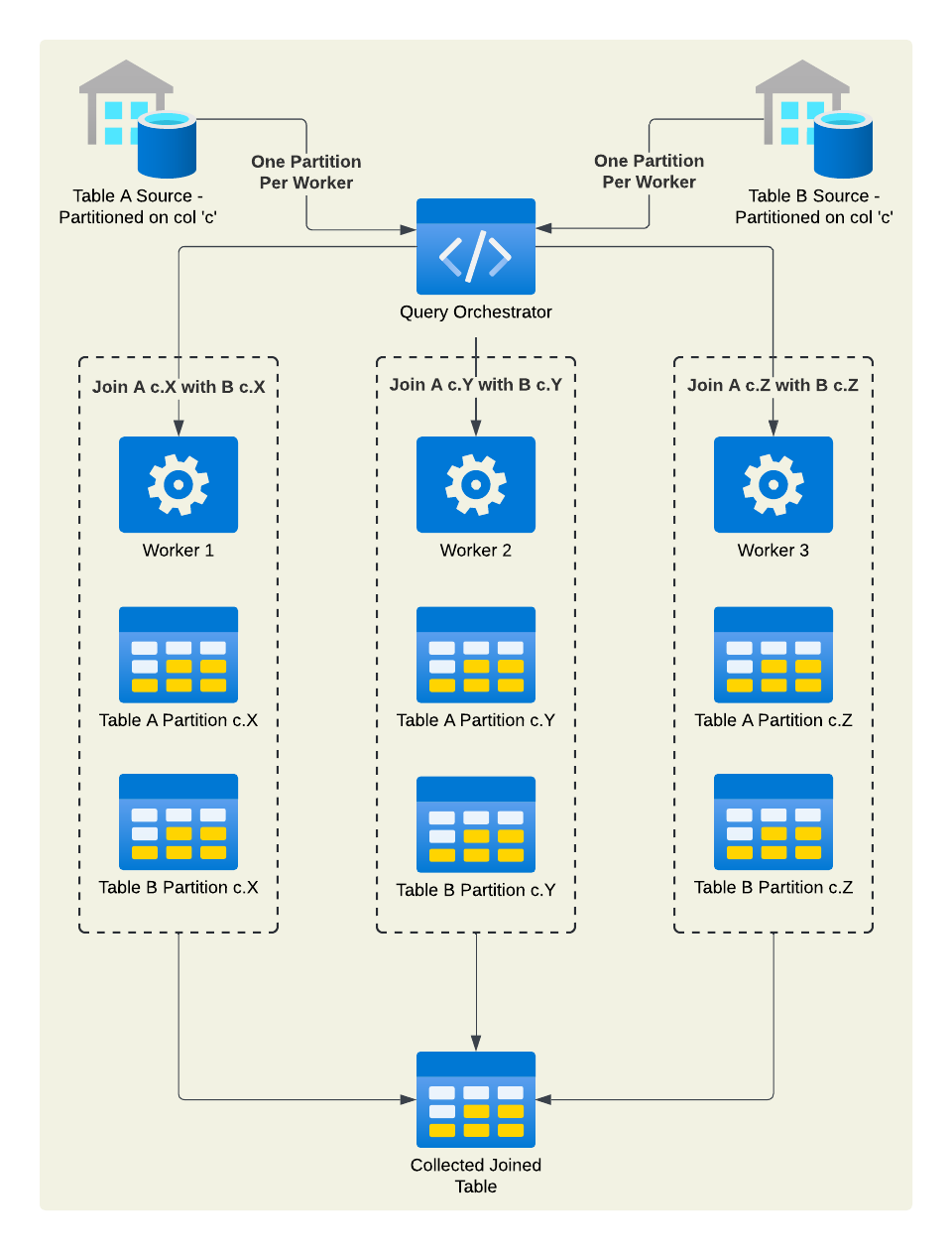
Co-located joins work if and only if two tables are being joined on the same field by which they were partitioned for storage. This allows worker nodes to operate on the same partitions of both tables in the same worker node, and avoids the need to shuffle data between nodes. In theory, this is faster than a broadcast join because no data needs to be replicated and broadcasted at all. However, the drawback is that this requires the original storage partition key to match the join key, which means it can only be used under very specific conditions.
When modelling a data lake or warehouse, having some prior knowledge about anticipated join queries on datasets can allow you to select good partition keys and maximize the chances of co-located joins.
Ideal Use Case
The partition keys for both tables match the join key.
Atleast one of the tables is not sorted (or indexed) by the join key (for sorted datasets, see sort merge joins).
Predicate Constraints
No strict constraints (same as broadcast joins).
Shuffle Hash Joins

In cases where the data being joined cannot be co-located, is not sorted by the key, and both tables being joined are large, the next best option is to use a shuffle hash join. Here is a simple breakdown of the steps involved in a shuffle hash join:
Step 1: Hash Partitioning: Both datasets are partitioned (shuffled) based on the hash value of the join key.
Rows with the same join key are sent to the same worker node. This is crucial for the subesquent steps.
Step 2: Build Hash Table: On each worker node, a hash table is built for the smaller partition.
Step 3: Probe Hash Table: The other partition is scanned, and for each row, its join key is looked up in the hash table. If a match is found, the rows are joined.
Shuffle joins are expensive operations due to the network overhead of shuffles. They are also particularly vulnerable to skewed join keys. However, they are an important pattern in distributed data joins when joining two large tables.
Ideal Use Case
Two large tables are being joined where neither would fit into a single node’s memory.
The data is neither sorted nor indexed on the join key.
The partition keys doesn’t match the join key for at least one table.
Predicate Constraints
At least one Equality Predicate: e.g.,
col1 = col2
Sort-Merge Joins

In any of the cases above, if the tables being joined are already sorted by the join key, a sort-merge join is likely the ideal strategy. This usually also applies if the tables are nearly pre-sorted by the join key (such that the cost of sorting them is low). In relational databases, indexed keys work just as well, since there will always be a data structure maintaining a sorted order of the index.
As the name suggests, there are two steps to a Sort-Merge join:
The datasets are sorted on the join key. This enables the next phase at O(n) time.
The sorted keys are then merged and the join conditions are applied. This can be broken down into the following steps:
Two pointers start scanning both sorted tables simultaneously from the 0th position.
The current row of both pointers are compared
Depending on whether the join condition (e.g., equality on join keys) is satisfied, rows are either joined or one pointer is advanced to continue the comparison.
Unlike our previous examples, the sort merge algorithm applies to single-server joins just as well. This affords a lot of flexibility to the query engine, which can partition and distribute both tables in ways that best optimize for the size and capacity of its worker nodes. The only constraint is that each partition should receive continous sets of key rows from both tables.
Ideal Use Case
Both tables are pre-sorted on the join keys.
Both tables are being joined on an indexed field or primary key.
Predicate Constraints
Sort merge joins are optimized for either of the following predicates:
Equality predicates: e.g.,
col1 = col2Range predicates: e.g.,
col1 BETWEEN 10 AND 20
Sort merge joins do not work well with inequality predicates since they not lend to a straightforward merge process.
Summary
Each distributed join strategy covered in this article comes with its own unique challenges and advantages. While modern query engines are usually capable of selecting the right join strategy based on its analysis of the query and data distribution, understanding the differences in how these join strategies operate will allow you to understand how your query engine operates under the hood. This is incredibly important knowledge for Data Platform Engineers who need to optimize query engines and clusters. Furthermore, frameworks like Spark allow you to manually configure join strategies, which is a powerful feature once you understand what is going on under the hood.
Further Readings
Performance Tuning on Spark (Discusses Spark’s implementation of Join Strategies)
Choosing the Right Join Algorithm (Schreiber on Clickhouse Engineering Blog)
Distributed Joins (Apache Ignite)
Advanced Join Strategies for Large-Scale Distributed
Computation (Bruno, Kwan, Wu at Microsoft)
A predicate in SQL joins is the operation in the ON clause, which dictates the key conditions on which the tables are joined.